How to make your data cumulative

For your bar chart race to display correctly, your data needs to be cumulative.

This means that the values in each row will build from left to right, with the next column's raw value being added to the sum in the last column. This can also be described as a sequence of partial sums of a given dataset or adding a summation of data as it grows with time.

If your bars are frantically jumping up and down the screen like in the below example, this is probably because your data isn't cumulative.

Luckily, this can be fixed rather quickly with some spreadsheet magic.

1

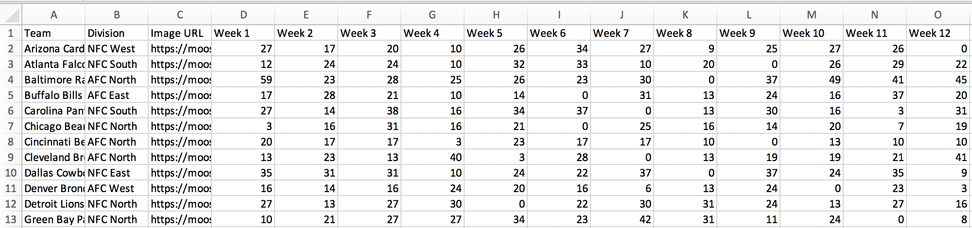
To get started, open your data in Excel or Google Sheets. We're using the data from the example above, which shows the points of football teams over 12 weeks. This data is in a "wide" format, in which each row contains multiple observations.



2

Next, to calculate the cumulative sum for numbers in row 2, we start a new row beneath the table and enter the following formula:

=SUM($D$2:D2)

In your running total formula, the first reference should always be an absolute reference with the $ sign ($D$2). Because an absolute reference never changes no matter where the formula moves, it will always refer back to D2. The second reference without the $ sign (D2) is relative and it adjusts based on the relative position of the cell where the formula is copied.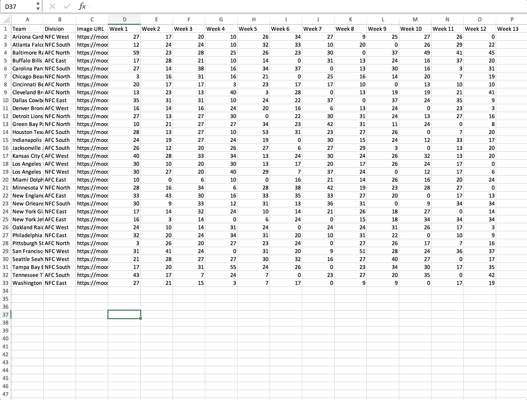



3

We can then copy this formula across the entire row. When our sum formula is copied to the next column, it becomes SUM($D$2:E2), and returns the total of values in cells D2 to E2. After that, the formula turns into SUM($D$2:F2), and totals numbers in cells D2 to F2, and so on.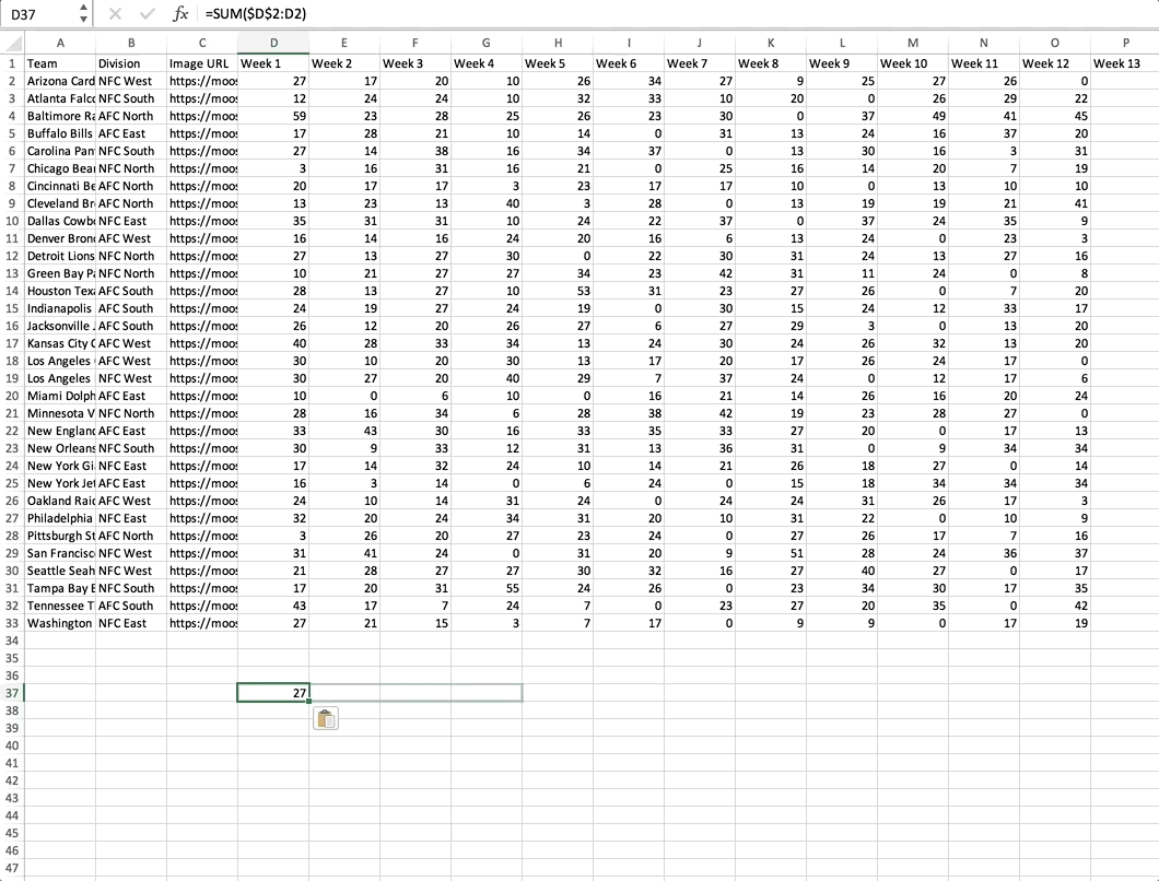



4

Repeat the same for the rest of the rows, replacing the first $D$2 with $D$3 all the way down to $D$33, and copy the formula across the rest of the rows to receive the cumulative data for all your rows.

5

Copy your data back into Flourish, and enjoy a much smoother Bar chart race experience!